UDC 550.34

https://doi.org/10.26516/2541-9641.2025.4.172

EDN: QCIPKI

From Icequake to Earthquake *

S.A. Bornyakov¹, A.A. Dobrynina¹, Y. Guo², L. Yao², A.N. Shagun¹, Y. Zhuo², V.A. Sankov¹, D.V. Salko¹, A.I. Miroshnichenko¹, A.A. Karimova^1,3

¹Institute of the Earth's Crust, Irkutsk, Russia

²Intitute of Geology of China Eartquake Administration, Beijing, China

³Irkutsk State University, Irkutsk, Russia

Abstract. There was performed instrumental deformation and seismic monitoring of the ice cover of Lake Baikal. Evidence was found for an autowave nature of ice deformations before icequakes. Autowave dynamics of deformations in the ice cover is a consequence of self-organization the ice cover as a structurally inhomogeneous medium in a critical state. The self-organization of the deformation process is confirmed by the results of processing the time series data by structural function curvature analysis method (SFCAM) and by spectral analysis method based on the Lomb-Scargl periodogram. The analysis of seismic monitoring data for the ice cover showed that the autowave processes are characterized by constant frequency 0.1 Hz.

The revealed features of the occurrence of deformations and microseismic vibrations of ice before ice strikes are compared with those identified previously for the occurrence of rock deformations before the last strong earthquakes in the southern Baikal region - Kultuk, Bystrinsky and Kudara. It is shown that as well as the icequakes, the earthquakes were preceded by self-organization of the deformation process. The self-organization of the deformation process and low-frequency autowave oscillations below and above 0.1 Hz, which occur before icequakes and earthquakes, can be considered as their inevitable precursors.

Keywords: icequake, earthquake, self-organization, precursor

Introduction

Ice has a wide range of mechanical properties and behaves either as an elastic-viscoplastic body or as an elastic body depending on the temperature and strain rate (Budd, 1989; Durham et. al., 2010; Petrovic, 2003). The deformation and destruction of ice are accompanied by seismic effects called "icequake" by analogy with tectonic earthquakes. The research of icequakes in glacier and sea ice has led to the emergence of a new seismological direction – cryoseismogy (Podolskiy and Walter, 2016). Seismological studies of glaciers are mainly aimed at studying their structure, internal deformations, and spatial displacements along the base. These studies have shown that the icequakes caused by glacier-related processes are divided into low-frequency and high-frequency events, with frequencies from 10⁻³ to 10² Hz and moment magnitudes from M^–3 to M⁷ (Podolskiy and Walter, 2016; Helmstetter, 2022; and others).

The main causes of icequakes are gravity and thermal expansion of ice. The first factor is constant and does not change over time. The second factor is seasonal and actively manifests itself in spring and summer when the air temperature rises. At the same time, the temperature of the glacier changes slowly due to its large volume, as a result of which the accumulation of high stresses, sufficient to generate icequakes therein, takes a long time.

There is a significant change in relation to ice-covered lakes in the regions with a sharply continental climate. An illustrative example is Lake Baikal (Fig. 1). Its small ice thickness averaging 0.8-1 m and sharp changes in spring temperatures from –5-10 °C at night to +5-10 °C during the day lead to rapid heating of the ice and a sharp increase in its volume due to thermal expansion and destruction with manifestation of seismic effects.

The mechanical behavior of the ice cover under slow deformations is similar to that of the lithosphere under long-term tectonic stresses (Dobretsov et. al., 2007, 2013; Ruzhich et. al., 2009). This suggests that the patterns of icequake preparation are also fitting with the preparation of earthquakes.

The authors carried out instrumental deformation and seismic monitoring of the ice cover of Lake Baikal in order to identify the patterns of icequake preparation and to verify those using tectonic earthquakes as an example.

Fig. 1. Location of Lake Baikal (a), test site location on the ice cover (b, c) and the layout of equipment thereon (d).

1 – permanent cracks; 2 – strain sensor; 3 – seismic station; 4 – directions of movement of the ice cover; 5 – epicenter of the Kudara earthquake.

Рис. 1. Расположение озера Байкал (a), расположение испытательного полигона на ледяном покрове (b, c) и расположение оборудования на нём (d).

1 – постоянные трещины; 2 – датчик деформации; 3 – сейсмическая станция; 4 – направления движения ледяного покрова; 5 – эпицентр землетрясения в Кударе.

Object of monitoring

In winter, the ice cover of Lake Baikal undergoes the formation of multi-kilometer permanent cracks which have opening-closing behavior with variations in negative air temperatures (Fig. 2 a, b). In spring, mainly in the first half of March, the daytime air temperature can rise to positive values. This is accompanied by a significant increase in the volume of the ice cover due to its thermal expansion and an increase in tangential compression stresses therein. Under the influence of these stresses, the contact between the ice plates in the permanent crack becomes broken, and one of the plates is pushed under the other (Fig. 2 b, d).

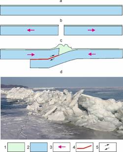
Fig. 2. A schematic representation of the formation of permanent shear fracture (b) in the ice cover (a) and its subsequent transformation into an underthrust during thermal expansion of ice (c). (d) a photograph of the underthrust zone formed in the ice cover of Lake Baikal. 1 – snow; 2 – ice; 3 – direction of movement of the ice plates; 4 – a periodic activation of the contact between the ice plates; 5 – direction of relative movement of the ice plates when there occurs an activation of contact therebetween.

Рис. 2. Схематическое изображение образования постоянного сдвигового раскола (b) в ледяном покрове (a) и его последующего превращения в подтолчок при тепловом расширении льда (c). (d) фотография зоны подтолка, образовавшейся в ледяном покрове озера Байкал. 1 – снег; 2 – лёд; 3 – направление движения ледяных плит; 4 – периодическая активация контакта между ледяными плитами; 5 – направление относительного движения ледяных плит при активации контакта между ними.

Underthrusting and the subsequent activation of periodically freezing contact between the ice plates by the "stick-slip" mechanism are accompanied by icequakes, what can be seen in the «video-ice». The preparation of icequakes, which takes place at small time intervals of a few hours, makes them a unique object for instrumental observations. The observed similarity between the mechanical deformation behavior of the ice cover and that of the lithosphere can provide useful information for the development of methods for moderate- and short-term prediction of tectonic earthquakes (Dobretsov et al., 2007, 2013; Ruzhich et al., 2009).

The object of monitoring was one of the permanent cracks, located 4 km from the shore in the southern Lake Baikal (coordinates 52^о31^/06.27^//; 106^о13^/06.72^//) (Fig. 1).

2. Experimental setups and processing methods

There were two types of instrumental monitoring of the ice cover performed near the underthrust: deformation and seismic.

2.1. Equipment for deformation monitoring

Deformation measurement was carried out using an instrumental complex (IC) (Bornyakov and Salko, 2016). The IC includes a data collection-transmission unit (DCTD), analog-to-digital converters (ADC), analog sensors, an autonomous power supply system (APSS), a remote base server, and client-server control software packages (Fig. 3). The IC is designed to receive deformation signals, take their accurate time-related measurements, compile a flash-memory dataset, and transfer the datasets to the remote base server via the on-line mobile communication system.

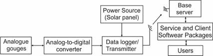
Fig. 3. A block diagram of the instrumental complex designed for deformation monitoring.

Рис. 3. Блок-схема инструментального комплекса, предназначенная для мониторинга деформаций.

The measuring element of the IC is a rod sensor with a base of 2 m. There were used six monitoring sensors. The sensors were installed 50 m apart from each other perpendicular to the direction of the permanent crack strike at a distance of 15 m therefrom (Fig. 4). The sensor was polled with a discreteness of 4 Hz.

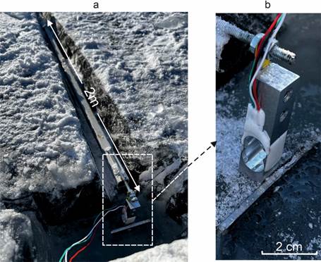
Fig. 4. A rod sensor frozen in the ice cover of Lake Baikal (a) and its enlarged fragment (b).

Рис. 4. Стержневой датчик, замороженный в ледяном покрове озера Байкал (a) и его увеличенный фрагмент (b).

2.2. Equipment for seismic monitoring

Seismic vibrations of the ice cover were recorded by Baikal-7HR seismic stations with SK-1 sensors (https://www. gsras/unu/uploads/files/Dataloggers/Bairal-7HR.pdf).

2.3. Methods of monitoring data processing

To process deformation monitoring data, there were used the spectral analysis (SPA) method based on the Lomb-Scargla periodogram (Lomb, 1976; Scargle, 1982, 1989; Savransky, 2023) and the structural functions curvature analysis method (SFCAM) (Vstovsky, 2006; Vstovsky and Bornyakov, 2010).

2.4. Methods of seismic data processing

The seismic data processing was performed by methods of spectral-time analysis (STAN) and polarization analysis of 30-minute periods in microseismic motion records. The STAN method is based on an estimate of current spectrum of the part of a signal corresponding to short-length sliding time window (the length was selected to be from 10 to 60 seconds). At such an estimate, the power spectrum of a signal occurs depending on both frequency and location (middle part or right edge) of the widow. The polarization analysis, or plotting the patterns of directional motion of the particles in seismic waves, is made in two planes: north-south – east-west (NS-EW) and horizontal – vertical (H-Z). The directional patterns show the predominant direction of particle motion in a medium and ones are also used to determine the type of a seismic wave.

Results

The main result of deformation monitoring was the detection of the autowave nature of ice deformations occurring before icequake (Fig. 5 a). Beginning some minutes or a few tens of minutes before the impact, this process develops with an increase in the amplitude of oscillations, often with a multiple reduction in their period (Fig. 5 b, c). Immediately before an icequake, such an orderly nature of oscillations changes to chaotic, with an increase in their amplitude and period. The periods of self-oscillations are 0.1-0.2 Hz.

Figure 6 and Figure 7 show the results of processing the deformation monitoring data by SFCAM and SPA methods, respectively. In the first case, the processing involved the data for March 8, 9, 10 and 11, when there occurred several strong icequakes (Fig. 6). In the second case, there was performed a processing of the data for March 7, with one strong icequake (Fig. 7).

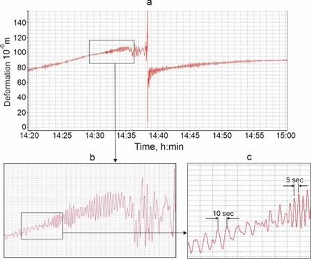
Fig. 5. An example of the autowave nature of ice deformations that occur before an ice strike (a) and its details (b, c).

Рис. 5. Пример автоволновой природы деформаций льда, происходящих перед ударом о лёд (a), и его детали (b, c).

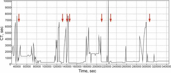
Fig. 6. A graph of variations of the correlation time parameter on March 8, 9, 10 and 11. The arrows mark the moments of occurrence of the most powerful icequakes.

Рис. 6. График вариаций параметра корреляционного времени на 8, 9, 10 и 11 марта. Стрелки отмечают моменты самых мощных ледяных землетрясения.

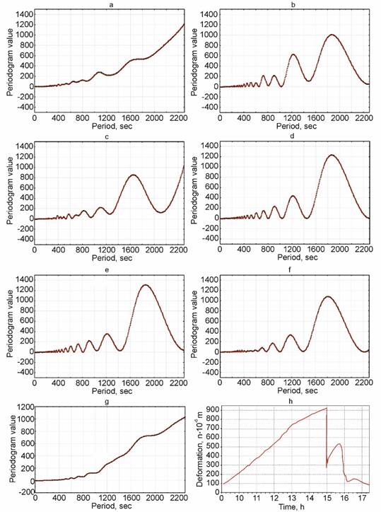
Fig. 7. Spectrograms of ice deformation time series from 09. 00 to 16.00 March 7, 2021 for hourly intervals: 09.00-10.00 (a); 10.00-11.00 (b); 11.00-12.00 (c); 12.00-13.00 (d); 13.00-14.00 (e); 14.00-15.00 (f); 15.00-16.00 (g). h – graphical representation of the initial data.

Рис. 7. Спектрограммы временных рядов деформации льда с 09.00 до 16.00 7 марта 2021 года для часовых интервалов: 09.00–10.00 (a); 10.00–11.00 (b); 11.00–12.00 (c); 12.00–13.00 (d); 13.00–14.00 (e); 14.00–15.00 (f); 15.00–16.00 (g). h – графическое представление начальных данных.

The results of seismic monitoring of the ice cover showed that variations in the level of fluctuations of the ice cover depend on the temperature of ice, which determines the level of stresses therein. Root-mean-square amplitudes of microseismic background at low air temperatures in the morning hours are an order of magnitude lower than those recorded in the day time when the temperature rises by 5–10 degrees.

In the morning hours, self-oscillations occur only in the horizontal plane with a period of 20-30 minutes, a frequency of approximately 0.1 Hz, and a pulse duration of 60÷150 seconds (Fig. 8). Unlike the horizontal component, the vertical does not show any pronounced self-oscillations and has a wide frequency range (0÷8 Hz.), though there is a weakly pronounced peak at a frequency of 0.1 Hz.

In the daytime, self-oscillations are well-pronounced in all three directions (Fig. 9 a). The spectral peaks, corresponding to the fundamental frequency of 0.1 Hz, are better pronounced (Fig. 9 b). In this case, the period of occurrence of self-oscillations is reduced to 5–15 minutes.

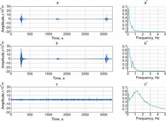
Fig. 8. An example of self-oscillations and their spectra in the morning time.

Рис. 8. Пример самоколебаний и их спектров утром.

Figure 9 shows an example of typical fluctuations of the ice cover and their daytime spectra before icequakes.

The graphs show well-pronounced self-oscillations occurring in all three directions (N-S, W-E, Z) with a frequency of 0.1 Hz.

At the moment of icequakes, the discharge of stresses in the ice cover leads to the occurrence of several large-amplitude oscillations with frequencies of 0.6÷1.2 Hz. The duration of oscillations is about 10 seconds. The examples of seismograms and their corresponding spectra for a single ice impact are shown in Figure 10.

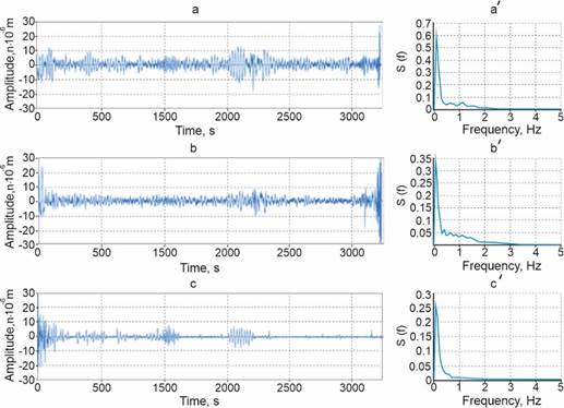
Fig. 9. An example of self-oscillations and their daytime spectra before icequakes. The graphs show pronounced self-oscillations in all three directions (N-S, W-E, Z) with a frequency of 0.1 Hz.

Рис. 9. Пример самоколебаний и их дневных спектров до ледяных толчков. Графики показывают выраженные самоколебания во всех трёх направлениях (N-S, W-E, Z) с частотой 0.1 Гц.

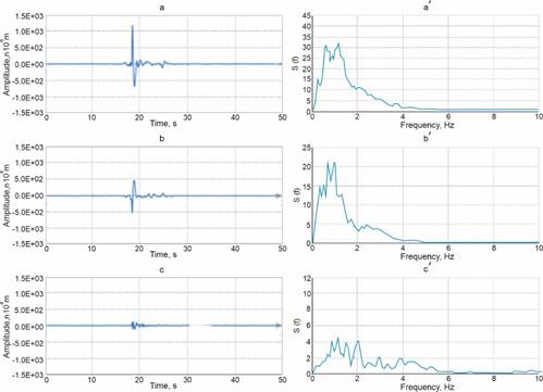
Fig. 10. An example of seismograms and their icequake-related spectra.

Рис. 10. Пример сейсмограмм и их спектров, связанных с ледяными землетрясениями.

4. Discussion

4.1. Basic concept to interpreting the icequake and earthquake preparation processes.

Studies of tectonic earthquake sources are mostly based on the concept of avalanche-unstable fracturing (AUF) (Myachkin, 1978) and the stick-slip model (Brace and Byerlee, 1966). The AUF model describes how numerous small ruptures occur and grow, then rapidly merge and form a long fault, and this process results in a seismogenic displacement along the fault. In contrast, the stick-slip model describes the process of periodic seismogenic activation of an existing fault. A similar process occurs during the icequake preparation.

In the investigations of large active continental lithospheric faults, the stick-slip mechanism is observed to occur more often than the unstable fracturing and thus given more attention in studies aimed at earthquake prediction. In the 1960–1990s, researchers performed numerous laboratory experiments using the stick-slip model to investigate and assess the recurrence of seismogenic displacements on faults. Physical phenomena preceding the displacements were recorded and analyzed in order to identify possible precursors of earthquakes. In combination with the findings from theoretical studies and field observations, the results of these experiments have significantly improved the understanding of the earthquake source physics and made it possible to propose and justify a wide range of short-term precursors (Cicerone et al., 2009), among which there was the anomalous behavior of geophysical parameters before an earthquake. However, many of these studies were based on outdated concepts and thus failed to solve the problem of earthquake prediction and forecasting. Furthermore, their results raised doubts on whether seismic forecasting was possible at all (Geller et al., 1997). Some progress has been achieved by using the concept of synergetics (Haken, 1978; Kondepudi and Prigogine, 1998), in terms of which a seismically active fault is an open nonequilibrium dynamic system; an earthquake is a self-organized criticality (SOC) (Bak and Tang, 1989); and a cooperative behavior is typical of the deformation process right before an earthquake (Crampin and Gao, 2013; Feder and Feder, 1991; Ciliberto and Laroche, 1994; Olami et al., 1992).

The SOC model has been confirmed in experiments using a precision servo-controlled press to simulate seismic activation of faults due to the stick-slip mechanism (Ma et al., 2012, 2014). According to their results, a loaded system of two blocks contacting along a rupture undergoes a multi-stage deformation process preceding the occurrence of a slip impulse.

These stages are marked by changes in the average shear stress over time (Fig. 1). The graph shows shear stress variations and illustrates the deformation dynamics of the entire boundary between the interacting blocks before the occurrence of the slip impulse (marked by a grey box at an interval of 660–700 sec, see the inset in Fig. 1). In segment N–O, the graph shows a deviation from linearity. At point O, the shear stress reaches its maximum value, and the system develops into the metastable state. In segment OAB₂, there occurs the achievement of a meta-instable state. It includes the early (AB₁) and late (AB₂) meta-instability substages. After point В₂, dynamic instability manifests itself as a slip impulse. In the first metastable stage, relative displacements of the blocks start and develop along with slow relaxation of the stresses accumulated at the interblock contact. This process takes place in the quasi-creep stationary mode, which is due to the occurrence of small micro-sources of destruction (i.e. small activated segments of the rupture). During the early meta-instability substage, the process of stress decrease continues slowly, and the isolated segments of the rupture continue gradually to increase. The late meta-instability substage is characterized by accelerated synergism – by deformation increase and acceleration. The synergism manifests itself immediately before the transformation of the quasi-static state into a dynamic one due to the cooperative behavior of all activated segments, which means their self-organization. It is reasonable to expect that in a natural setting, the meta-instable stage of activation of a fault can be detected by the self-organization of its segments.

Thus, the stick-slip model in its synergistic interpretation (Ma et al., 2012, 2014) demonstrates that the critical dynamic state of a fault (which is achieved at the late meta-instability substage) should be investigated in detail as a potential earthquake precursor rather than any anomalous variations of one or another geophysical parameter of the fault. A direct and inevitable indicator of the critical dynamic state (i.e. the meta-instability substage) is self-organization of activated fault segments at the fault plane immediately before seismogenic rupturing of a certain fault. Considering natural faults, we suggest that the self-organization process can be diagnosed by processing the time series of rock deformation signals. We have tested this research approach by spectral analysis (Scargle, 1982, 1989; Savransky, 2023; Bornyakov et al., 2017, 2022) and the structural functions curvature analysis method (SFCAM) (Vstovsky, 2006; Vstovsky and Bornyakov, 2010; Bornyakov et al., 2022).

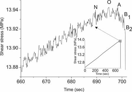
Fig. 11. Shear stress vs time before the slip impulse (after (Ma et al., 2014)). Inset (right corner) – linear graph of the shear stress increase; the slip impulse is marked by a grey box.

Рис. 11. Сдвиговое напряжение против времени до импульса скольжения (после (Ma и др., 2014)). Вставка (правый угол) — линейный график увеличения сдвигового напряжения; Импульс скольжения отмечен серой рамкой.

4.2. Autowave dynamics as an indicator of the process of self-organization of deformation process in the ice cover

The autowave dynamics of deformations of the ice cover is due to its ability for self-organization, as well as that of any other open, non-equilibrium, and structurally inhomogeneous system (Haken, 1978; Kondepudi and Prigogine, 1998). The modeling results known so far (Sobolev and Ponomarev, 2003) and the results of instrumental observations of deglaciation in mountainous areas (Pralong, 2006), demonstrating the autowave dynamics of deformations of such structurally inhomogeneous systems, subjected to stresses close to the ultimate strength, allow us to consider a similar phenomenon we have recorded to be natural, unrelated to the peculiarities of the deformation of the lake ice cover but linked to the ability of these systems for self-organization in such a critical state (Haken, 1978; Kondepudi and Prigogine, 1998).

The self-organization of the deformation process in the ice cover is confirmed by the results of processing time series of deformations by SFCAM and SPA methods (Fig. 6, 7). As noted above, both methods allow these deformation series to yield the time intervals of their-correlated behavior of the parameter under analysis, that is, the intervals in which there occurred self-organization of the deformation process.

In the first case, such intervals correspond to a sharp increase in the parameter of "correlation time" (CT) (Fig. 6). As can be seen from the graph, most of the strongest icequakes are preceded by the manifestation of self-organization of the deformation process, coinciding with the time of occurrence of self-oscillations.

In the case of spectral analysis, the time intervals of self-organization occurrence correspond to an ordered form of a spectrogram reflecting the correlated nature of oscillations of different periods in the deformation process (Fig. 7 d, e, f). Beyond these intervals, spectrograms are chaotic in nature (Fig. 7 a, b, c).

The results of deformation and seismic monitoring of the ice cover of Lake Baikal as a whole show that the peculiarities of icequake preparation correspond to the above-described "stick-slip" model in its synergistic interpretation. An important and inevitable element of this preparation is self-organization of the deformation process at the meta-unstable stage. Thus, self-organization of the deformation process can be considered as its inevitable precursor.

4.3. Similarity of deformation processes before icequakes and earthquakes

The revealed features of the occurrence of deformations and microseismic vibrations of ice before ice strikes are compared with the previously identified features of the occurrence of rock deformations before the last three strong earthquakes in the southern Baikal region (Bornyakov et al., 2022). The comparison was based on the results of spectral analysis of deformation and seismic monitoring data obtained from the geodynamic test site "Talaya" before the Kultuk (27.08.2008, M = 6.3) and Bystrinsky (21.09.2020 M = 5.4) earthquakes and from the geodynamic test site "Buguldeika" before the Kudara earthquake (09.12.2020, Mw = 5.5) (Fig. 1).

4.3.1. The Mw 6.3 Kultuk earthquake of August 27, 2008

The rock deformation monitoring data from the Talaya test site for the year of 2008 were processed to characterize the Mw 6.3 Kultuk earthquake that occurred on August 27, 2008 at the southwestern termination of Lake Baikal. The data were processed by SFCAM and SPA methods. The result of data processing by these methods is shown in Figure 12. As noted above, a sharp increase in the ST parameter indicates the development of self-organization in the analyzed deformation process. As shown in the figure, sharp CT changes are observed approximately 65000–70000 minutes (45–50 days) before the Kultuk earthquake. The range of these changes is wide, from 1000 to 10000 minutes (Fig. 12). Two peak CT values in time interval 273000–285000 minutes (i.e. within 8 days) indicate two episodes of the appearance and failure of temporary interrelations in the deformation process, which most probably resulted from a significant re-arrangement of stress fields in the fault-block structure of the lithosphere, specifically in the focal area, which caused the earthquake. In this case, we can say that a mid-term (45–50 days) precursor of the Kultuk earthquake has been reliably detected from the rock deformation monitoring data.

Approximately one month (40000–45000 minutes) before the earthquake, the focal area is in the metastable state, CT=100–200 minutes. A sharp CT increase is observed ten days (14700 minutes) before the earthquake. The CT value is further increased and reaches 6200 minutes six days (336000 minutes) before the earthquake (Fig. 12). This time point can be interpreted as the beginning of the early meta-instability substage, when previously close interrelation in the deformation process begins to fail. This failure develops up to the time point of 340500 minutes. The beginning of a short-term recovery of the interrelation (three days before the earthquake) is the beginning of the late meta-instability substage.

Thus, the above SFCAM results show that CT variations reflect the features of the deformation process that develops in the fault-block medium, wherein a source of an imminent earthquake is developing. In particular, an anomalous growth of CT values is an indicator of the development of temporary interrelations in the time series of the deformation data, which result from the self-organization of the deformation process. In case of the Kultuk earthquake, the self-organization took place twice – a month and a few days before the seismic event. These two episodes of self-organization were, respectively, mid- and short-term earthquake precursors.

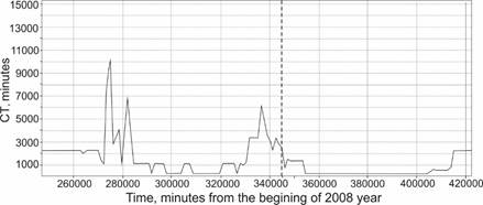
Fig. 12. Correlation time (CT) variations according to the data of sensor 3 (Talaya point). The time coordinate is given in minutes from the beginning of the year. The earthquake beginning (344732 minutes from the start of the year) is marked by a dashed line.

Рис. 12. Изменения корреляционного времени (CT) в зависимости от данных датчика 3 (точка Талайя). Временная координата указывается в минутах с начала года. Начало землетрясения (344732 минут с начала года) отмечено пунктирной линией.

For a spectral analysis, the rock deformation monitoring data collected from June 10 to October 09, 2008 were grouped into five datasets: June 10 – July 09 (A), July 10 – August 09 (B), August 10 – August 26 (pre-seismogenic time) (C), August 28 – September 09 (D), and September 10 – October 09, 2008 (E) (Fig. 13). It should be noted here that signals recorded on August 27, 2008 (earthquake date) were excluded from the analysis. Spectrograms clearly show that both the structure and the intensity of the oscillations change with time, especially in the range from E5 to 8E5 (Fig. 13), as follows:

June 10 – July 09 (Fig. 13 a): Six main periods of oscillations; the oscillation pattern is chaotic.

July 10 – August 09 (Fig. 13 b): Nine main periods; periodogram parameter 24hP begins to decrease; the oscillation pattern has an element of order.

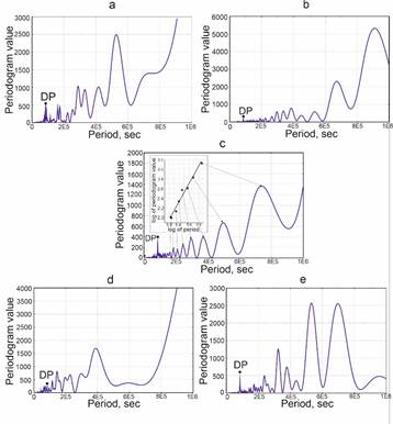
Fig. 13 Spectral analysis results for the five rock deformation datasets: (a) June 10 – July 09; (b) July 10 – August 09; (c) August 10 – August 26; (d) August 28 – September 09; (e) September 10 – October 09, 2008. DP – periodogram parameter (24-hours period).

Рис. 13 Результаты спектрального анализа для пяти наборов данных по деформации горных пород: (a) 10 июня – 9 июля; (b) 10 июля – 9 августа; (c) с 10 по 26 августа; (d) 28 августа – 9 сентября; (e) 10 сентября – 9 октября 2008 года. DP – параметр периодограммы (24-часовой период).

August 10 – August 26 (Fig. 13 c): Pre-seismogenic state; parameter 24hP continues to decrease; the oscillation pattern is of a high degree of order, as shown by its fractal structure (see the inset). This means that the rock deformation data in this time series are in a close temporary interrelation, and the oscillations are time-coordinated and intensity-adjusted. Here, we reveal a consequence of the self-organization of the deformation process before the earthquake, which is supported by the above-described SFCAM results (Fig. 12).

August 28 – September 09 (Fig. 13 d): After the earthquake, there are significant changes in the rock deformation mode – the deformation process is very chaotic; parameter 24hP is increased; short- and mid-period (0–4Е5 sec) oscillations are dominant, and any long-period (4Е5 to 1Е5 sec) oscillations are lacking (or poorly pronounced).

September 10 – October 09 (Fig. 13 e): the deformation process tends to return to the original mode – this spectrogram is qualitatively similar to that for June 10 – July 09 (Fig. 13 a).

The analysis of the spectrograms with the focus on parameter 24hP reveals a specific pattern of its changes. In the spectrogram for June 10 – July 09, it is at the level of 600 minutes (Fig. 13 a). During two time intervals before the earthquake, it decreases to 350–400 minutes (Fig. 13 b, c). It remains at the same level for two weeks after the earthquake (Fig. 13 d), and then increases again (Fig. 13 e).

4.3.2. The Mw 5.4 Bystrinskoe earthquake of September 31, 2020

The deformation monitoring data obtained in Talaya point are in the time interval from 01.02. 2020 to 30.10.2020. The results of this data processing by the SFCAM method are shown in Figure 14. The graph shows that the process of deformation self-organization took place within 18 days before the Bystrinsky earthquake (T = 5200h)). During the final stage of its preparation, which began at T = 5558h, such self-organization was faster-moving in nature, most intensively manifested three days before it (Fig. 14).

The time series dataset (period from June 01 to October 30) was divided into intervals: June 1-30 – July 1-31, July 1-10 – August 1-31, September 1-20 – September 22-30 – October 1-30, with the spectral analysis performed for each sample (Fig. 15). These spectrograms show that the structure and the intensity of the oscillations vary over time, which is most clearly manifested for the periods within the range of their values from E5 to E6. On the first spectrogram in this interval, there are four main periods with the "periodogram" parameter values of more than 1000 (Fig. 15 a). In the next time interval, the number of the main periods increases to five due to the appearance of an additional period of 1.6E6. At the same time, the values of the "periodogram" parameter increase twice against the background of increasing randomization of the spectrogram (Fig. 15 b).

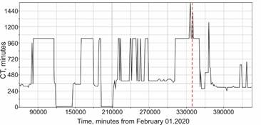
Fig. 14. A graph showing the variation of correlation time. A bold vertical dotted line marks the moment of the Bystrinsky earthquake. The time is shown in minutes of February 01, 2020.

Рис. 14. График, показывающий изменение времени корреляции. Жирная вертикальная пунктирная линия отмечает момент Быстринского землетрясения. Время показано в минутах на 1 февраля 2020 года.

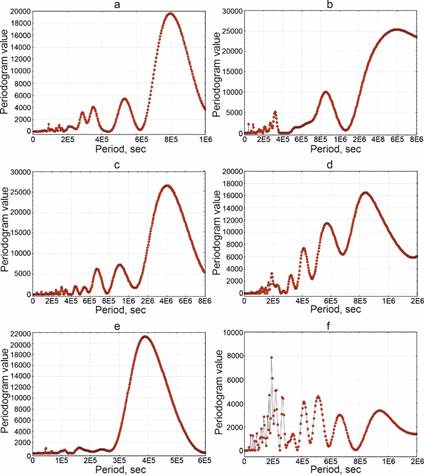
Fig. 15. Spectral analysis results for the six rock deformation datasets for Talaya point: (a) 1-30 June; (b) 1-31 July; (c) 1-31 August; (d) 1-20 September; (e) 22-30 September; (f) 1-30 October 2020.

Рис. 15. Результаты спектрального анализа шести наборов данных по деформации пород для точки Талая: (a) 1-30 июня; (b) с 1 по 31 июля; (c) с 1 по 31 августа; (d) 1-20 сентября; (e) с 22 по 30 сентября; (f) 1-30 октября 2020 года.

In the third interval, the number of the main periods of oscillations with the "periodogram" parameter values of more than 1000 increases to eight, and the structure of the spectrogram shows orderliness (Fig. 15 c), similar to that in Figure 7 d, e. In the subsequent, pre-seismogenic interval, this orderliness remains unchanged against the background of more than two times increase in the "periodogram" parameter (Fig. 15 d). After the earthquake, the spectrum is restructuring. In the last decade of September, only the large-period oscillation of 4E5 remains significant (Fig. 15 e). In the subsequent calculation period, there is a large decrease in the "periodogram" parameter, and the spectrogram has a disordered structure with short-period oscillations of predominant importance (Fig. 15 e).

4.3.3. The Мw 5.6 Kudara earthquake of December 10, 2020

The geodynamic polygon "Buguldeika" began operating at the end of August 2020. The short time series obtained by the time of the Kudara earthquake could not be processed by the SFCAM method.

The spectral analysis was made on the data obtained from September 2020 to January 2021. The entire time series was divided into the following intervals: September 1-30 – October 1-31, November 1-30, December 1-9, December 11-31, and January 1-31 (Fig. 16). These spectrograms show that the structure and the intensity of the oscillations vary over time, especially in the periods from E5 to E6. On the first spectrogram, in the range of values 2E5 – 7E5, there are only two main periods with the "periodogram" parameter values of more than 1000 (Fig. 16 a). In the next time interval, the number of the main periods increases to nine due to the manifestation of seven additional main periods of oscillations in the range of their values from 3E5 to 1.6E6.

At the same time, the values of the "periodogram" parameter increase more than twice; the spectrogram itself acquires a generally ordered structure (Fig. 16 b). In the third interval, the structure of the spectrogram as a whole remains unchanged, with a slight decrease in the "periodogram" parameter for certain periods (Fig. 16 b). The structural orderliness, typical of the pre-seismogenic state, is absent on the next spectrogram obtained during a 10-day period preceding the earthquake. There are no periods with values greater than 2.2E5, and the periods in the range of smaller values are three-four times as significant as those in the previous spectrograms (Fig. 16 b, c, d). It is noteworthy that meaningful fluctuations in this time interval are those with a daily period (Fig. 16 d). After the earthquake, the spectrum is restructuring. In the last two decades of December and in January, there is a gradual increase in the number of large-period oscillations and an increase of the "periodogram" parameter (Fig. 16 d, e). At the same time, the structure of spectrograms remains chaotic.

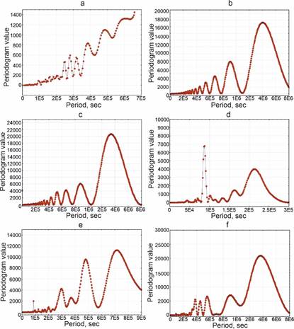
Fig. 16. Spectral analysis results for the six rock deformation datasets from Buguldeika point: (a) 1-30 September; (b) 1-31 October; (c) 1-30 November; (d) 1-20 September 09; (e) 22-30 September; (f) 1-30 October 2020.

Рис. 16. Результаты спектрального анализа шести наборов данных по деформации горных пород с точки Бугулдейка: (a) 1-30 сентября; (b) с 1 по 31 октября; (c) с 1 по 30 ноября; (d) 1-20 сентября 209 года; (e) с 22 по 30 сентября; (f) 1-30 октября 2020 года.

4.4. Similarity of seismic processes before icequakes and earthquakes

Spectral analysis of the data from seismic stations showed that before the icequake there are self-oscillations in the ice cover with a frequency of 0.1 Hz (Fig. 17). Taking into account this result, the analysis was carried out on the data recorded by the seismic station at the geodynamic test site "Buguldeika" before and after the Kudara earthquake.

The analysis of microseismic noise in the range from 0.01 to 1 Hz revealed a periodic increase in the amplitudes of oscillations in horizontal components in the frequency range of 0.01–0.1 Hz for the period of 10 to 4 days after the earthquake. 14 hours before and 9 hours after the earthquake, the amplitudes of oscillations increased to a maximum of 19.5 times relative to the quiet background (Fig. 17).

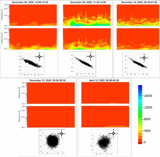
Fig. 17. Spectrograms and polarization diagrams of microseismic noise in the frequency range of 0.01–1 Hz recorded at the Kuyada station before and after the Kudara earthquake.

Рис. 17. Спектрограммы и диаграммы поляризации микросейсмического шума в диапазоне частот 0.01–1 Гц, записанные на станции Куяда до и после землетрясения Кудара.

Polarization analysis of microseismic noise revealed a clearly defined southeastward orientation of oscillations (mean azimuth – 121º), which is in good agreement with the azimuth to the epicenter of the main shock – 124.6º. Analysis of seismograms for the previous period (from December 1) and 10 hours after the Kudara earthquake did not reveal such effects in the field of microseimic noise.

Thus, the above results suggest that low-frequency self-oscillations recorded before the icequake also took place before the Kudara earthquake. This allows us to consider them as a stable process that precedes the dynamic displacement along the seismogenerating rupture / fault.

Conclusion

The instrumental deformation and seismic monitoring of the ice cover of Lake Baikal revealed an autowave nature of occurrence of ice deformations before icequakes. Autowave dynamics of deformations of the ice cover is a consequence of its self-organization as a structurally inhomogeneous medium in a critical state. The self-organization of the deformation process is confirmed by the results of the time series dataset processing with the SFCAM and SPA methods. The analysis of the seismic monitoring data for the ice cover showed that self-oscillations are characterized by constant frequencies of 0.1 Hz, and their amplitude increases with the increase in ice cover stresses.

The results of deformation and seismic monitoring of the ice cover are compared with similar results obtained at geodynamic polygons. It is shown that the revealed features of occurrence of deformations in the ice cover before icequakes are also found in the deformations of rocks before strong earthquakes. That is, the self-organization of the deformation process takes place before each earthquake, which is reflected in the variations of the ST parameter (Fig. 6, 12, 14) and the ordered form of spectrograms (Fig. 7, 13, 15, 16), and in the occurrence of low-frequency self-oscillations with increasing amplitude (Fig. 17). The stable manifestation of self-organization of the deformation process and low-frequency self-oscillations before icequakes and earthquakes allows us to consider them as short-term precursors of an approaching seismic event.

Author contributions

SAB, AAD and VAS analysed the results, prepared and revised the manuscript. ANS performed seismic monitoring and processed the results. AAD performed processing of microseisms before the Kudara earthquake. SDV performed strain monitoring. AIM performed spectral analysis of strain monitoring data. VGV and AES processed deformation monitoring data by SFCAMAS.

Competing interests

The contact author has declared that none of the authors has any competing interests.

Highlights

Before icequake and earthquake there is a self-organization of the deformation process;

low-frequency autowave oscillations are a sign of self-organization of the deformation process;

Self-organization of the deformation process is an inevitable precursor of an earthquake.

Acknowledgements and financial support

The work was conducted using the large-scale research facilities "South-Baikal instrumental complex for monitoring hazardous geodynamic processes" of the Center for Geodynamics and Geochronology at the Institute of the Earth's Crust, Siberian Branch of the Russian academy of Sciences.

This work was supported by the Ministry of Science and Higher Education of the Russian Federation, grant No. 075-15-2020-787 for implementation of major scientific projects on priority areas of scientific and technological development (project «Fundamentals, methods and technologies for digital monitoring and forecasting of the environmental situation on the Baikal natural territory»).

References

Bak P, Tang C (1989) Earthquakes as a self-organized critical phenomenon. Journal of Geophysical Research 94 (B11):15635–15637

Bornyakov SА et al. (2017) Diagnostics of meta-instable state of seismically active fault. Geodynamics & Tectonophysics 8 (4):989–998. doi:10.5800/GT-2017-8-4-0328.

Bornyakov SA et al. (2022) New approach to strong earthquake prediction in the south Baikal region on the basis of rock deformation monitoring data: methodology and results. Geodynamics & Tectonophysics 13 (2), 0588. doi:10.5800/GT-2022-13-2-0588

Bornyakov SA, Salko DV (2016) Instrumental deformation monitoring system and its trial in open-pit diamond mine. J of Mining Science 52(2):388-393.

Brace WF, Byerlee JD (1966) Stick-slip as a mechanism for earthquake. Science 153: 990–992.

Budd WF, Jacka TH (1989) A review of ice rheology for ice sheet modelling. Cold Regions Science and Technology 16:107–144.

Cicerone RD, Ebel JT, James Britton J (2009) A systematic compilation of earthquake precursors. Tectonophysics 476:371–396

Ciliberto S, Laroche C (1994) Experimental evidence of self-organization in the stick-slip dynamics of two rough elastic surface. J. Phys. I France 4:223-235. https://doi.org/10.1051/jp1:1994134

Crampin S, Gao Y (2013) The new geophysics. Terra Nova 25 (3):173–180. doi: 10.1111/ter.12030

Dobretsov NL et al. (2007) Ice cover of lake Baikal as a model for studying tectonic processes in the Earth's crust. Doklady Earth Science 413 (2):155–159.

Dobretsov NL et al. (2013) Advance in earthquake prediction by physical simulation on Baikal ice cover. Physical Mezomechanics 16 (1):52–61.

Durham WB et al. (2010) Rheological and thermal properties of icy materials. Space Science Reviews 153:273–298.

Feder JS, Feder J (1991) Self-organized criticality in stick-slip process. Physical Review Letters 66 (20):2669–2672.

Geller RG et al. (1997) Earthquake cannot be predicted. Science 275:1616–1617.

Haken Н (1978) Synergetics. An introduction. Nonequilibrium phase transitions in physics, chemistry and biology, Berlin; New York: Springer-Verlag, 355 p. urn:lcp:synergeticsintro0000hake:epub:ae913d9b-8018-4229-af98-327e116d163c

Helmstetter A (2022) Repeating low-frecuence isquakes in Mount-Blanc massif triggered by snowfalls. Journal of Geophysical Research: Earth Surface 127, e2022JF006837. https://doi.org/10.1029/22JF006837

Kondepudi D, Prigogine I (1998) Modern thermodynamics: from heat engines to dissipative structures. Modern thermodynamics: from heat engines to dissipative structures. John Wiley: Chichester, UK. 486 p.

Lomb NR (1976) Least-squares frequency analysis of unequally spaced data. Astrophysics and Space Science 39:447-462. https://doi.org/10.1007/BF00648343.

Ma J, Guo Y, Sherman SI (2014) Accelerated synergism along a fault: a possible indicator for an impending major earthquake. Geodynamics and Tectonophysics 2:87–99.

Ma J, Sherman SI, Guo YS (2012) Identification of meta-instable stress state based on experimental study of evolution of the temperature field during stick-slip instability on a bending fault. Science China Earth Sciences 55:869–881.

Myachkin VN (1978) Earthquake Preparation Processes. Moscow: Nauka, 232 p.

Olami Z, Feder HJS, Christensen K (1992) Self-organized criticality in a continuous, nonconservative cellular automaton modeling earthquakes. Physical Review Letters 68(8):1244–1247.

Petrovic JJ (2003) Review mechanical properties of ice and snow. Journal of Materials Science 38(1):1-6. doi: 10.1023/a:1021134128038

Podolskiy EA, Walter F (2016) Cryoseismology. Reviews of Geophysics 54:708-758. https://doi.org/10.1002/2016RG000526

Pralong A (2006) Oscilations in critical shearing: applications to fractures in glaciers. Nonlin. Processes Geophys 13:681-683

Ruzhich VV et al. (2009) Deformations and seismic phenomena in the ice cover of Lake Baikal. Russian Geology and Geophysics 50(3):207–214.

Savransky D. (2023). Lomb (Lomb-Scargle) Periodogram (https://www.mathworks.com/matlabcentral/fileexchange/20004-lomb-lomb-scargle-periodogram), MATLAB Central File Exchange. Retrieved November 3, 2023.

Scargle JD (1982) Studies in astronomical time series analysis. 2. Statistical aspects of spectral analysis of unevenly spaced dat. The Astrophysical Journal 263:835–853.

Scargle JD (1989) Studies in astronomical time series analysis. 3. Fourier transforms. Autocorrelation function and cross-correlation functions of unevenly spaced data. The Astrophysical Journal 343:874–887. https://doi.org/10.1086/167757.

Sobolev GA, Ponomarev AV (2003) Physics of earthquakes and precursors. Moscow: Nauka, 270 pp.

Vstovsky GV (2006) Factual revelation of correlation lengths hierarchy in micro- and nanostructures by scanning probe microscopy data. Mater. Sci. 12 (3):262–270.

Vstovsky GV, Bornyakov SA (2010) First experiences of seismodeformation monitoring of Baikal rift zone (by the example of South-Baikal earthquake of August 27, 2008). Natural hazards and Earth System Sciences 10:667–672.

 

Bornyakov Sergey Alexandrovich,

Candidate of Geological and Mineralogical Sciences,

664033, Irkutsk, Lermontov st., 128,

Institute of the Earth's Crust SB RAS,

Leading Researcher,

tel.: (3952)42-63-81,

еmail: bornyak@crust.irk.ru

 

Dobrynina Anna Alexandrovna,

Ph. Doctor in Geology,

664033, Irkutsk, Lermontov st., 128,

Institute of the Earth's Crust SB RAS,

Leading Researcher,

tel.: (3952)42-60-00,

email: dobrynina@crust.irk.ru

 

Zhuo Yanqun,

Ph. Doctor,

China, 100029, Beijing, Chaoyang District,

Hua Yan Li, Yard No. 1,

Institute of Geology, China Earthquake,

Administration,

Associate Researcher,

tel.: +86(10)62009112

 

Yao Lu,

Ph. Doctor,

China, 100029, Beijing, Chaoyang District,

Hua Yan Li, Yard No. 1,

Institute of Geology, China Earthquake,

Administration

Researcher,

tel.: +86(10)62009112,

email: guoysh@ies.ac.cn

 

Shagun Artem Nikolaevich,

664033, Irkutsk, Lermontov st., 128,

Institute of the Earth's Crust SB RAS,

Leading Engineer,

tel.: (3952)42-58-23,

email: shagun@crust.irk.ru

 

Zhuo Yanqun,

Ph. Doctor,

China, 100029, Beijing, Chaoyang District,

Hua Yan Li, Yard No. 1,

Institute of Geology, China Earthquake,

Administration,

Associate Researcher,

tel.: +86(10)62009112,

email: zhuoyq@ies.ac.cn

 

Sankov Vladimir Anatolyevich,

Ph. Doctor in Geology

664033, Irkutsk, Lermontov st., 128,

Institute of the Earth's Crust SB RAS,

Head of the Laboratory of Modern Geodynamics,

tel.: (3952)42-79-03,

email: sankov@crust.irk.ru

 

Salko Denis Vladimirovich,

664033, Irkutsk, Lermontov st., 128,

Institute of the Earth's Crust SB RAS,

Leading Engineer,

tel.: (3952)42-58-23,

еmail: denis@salko.net

 

Miroshnichenko Andrei Ivanovich,

Candidate of Geological and Mineralogical,

Sciences,

664033, Irkutsk, Lermontov st., 128,

Institute of the Earth's Crust SB RAS,

Senior Researcher,

tel.: (3952)36-95-62,

еmail: mai@crust.irk.ru

 

Karimova Anastasia Alekseevna,

Candidate of Geological and Mineralogical Sciences,

664033, Irkutsk, Lermontov st., 128,

Institute of the Earth's Crust SB RAS,

Junior Researcher,

664003, Irkutsk, Karl Marx st., 1,

Irkutsk State University,

Associate Professor,

tel.: (3952)42-63-81,

еmail: geowomen_nasty@mail.ru

 

Read the full article (English)